The 4+1D Discontinuous Galerkin Engine
DraftingA spectral numerical-relativity solver for a five-dimensional bulk
preprint — not yet on arXiv gr-qc (cross-list: physics.comp-ph) updated 2026-09-09
Abstract. We present a discontinuous Galerkin (DG) spectral-element solver for generalized-harmonic numerical relativity in 4+1 spacetime dimensions, targeting a hypercubed-sphere domain (eight cubed-sphere wedges per radial shell) with Legendre–Gauss–Lobatto collocation, upwind penalty fluxes at inter-element faces, fourth-order Adams–Bashforth time integration, and a Hesthaven–Warburton modal exponential filter for high-mode control. The vacuum and generalized-harmonic (GH) pipeline is validated end-to-end on a single GPU (sm_120 Blackwell tested), with bit-equality enforced between CPU and GPU kernel evaluations to a per-kernel tolerance of 1e-13 and an end-to-end pipeline tolerance of 1e-12. No finite-difference stencils are used anywhere in the solver; all spatial derivatives are spectral. This paper documents the solver's architecture and its validation methodology — it makes no claim about the physics content (matter sector, brane, or birth mechanism) evolved on top of it; those are the subject of the four papers that follow.
What this paper is, in plain language
Numerical relativity means solving Einstein’s equations on a computer — turning curved spacetime into numbers a machine can update, step by step, without the equations blowing up or drifting away from being a valid solution. This paper documents the tool that makes that possible for the WHD program: a solver built from scratch to evolve a five-dimensional spacetime (four space dimensions plus time), because the WHD picture needs a bulk with one more spatial dimension than the universe we experience.
Why spectral, not finite differences
Most numerical-relativity codes chop space into a grid and estimate derivatives from nearby grid points (“finite differences”). This solver does something different: on each small patch of the domain, a field is represented as a sum of smooth polynomial basis functions (a Legendre spectral expansion), and derivatives are computed exactly for that representation — not estimated from neighbors. For smooth solutions, this converges to the right answer far faster as resolution increases. The solver has no finite-difference code path anywhere; every derivative, everywhere, is spectral.
The domain: a hypercubed sphere
A five-dimensional ball is awkward to cover with a single coordinate patch — coordinate singularities pile up at the center and the usual angular coordinates misbehave near the poles. The solver instead builds the spatial domain out of eight “cubed-sphere” wedges (the same trick flight-simulation and climate codes use to tile a sphere with distortion-minimized squares) stacked in concentric radial shells. Each wedge is itself broken into spectral elements, and elements talk to their neighbors across shared faces using an upwind penalty flux — a scheme that lets information flow the right direction physically while keeping the whole assembly numerically stable.
Keeping high-frequency noise from taking over
Spectral methods are extremely accurate, but they are also prone to a specific failure mode: numerical noise piling up in the highest-frequency modes the discretization can represent, eventually swamping the real signal. The solver applies a modal exponential filter — a well-established technique (Hesthaven & Warburton) that gently damps the highest modes on a regular cadence without touching the smooth, physically meaningful part of the solution.
How we know it’s right
Two separate kinds of check matter here, and this paper keeps them distinct. First, does the GPU implementation compute the same thing as the CPU implementation? We require bit-for-bit equality (not “close enough”) for individual kernels, and agreement to 1 part in 10¹² for the full evolution pipeline over many time steps — a much stronger bar than typical floating-point tolerance, chosen because it turns “did I introduce a bug porting this kernel to the GPU” into a yes/no question instead of a judgment call. Second, and separately, does the solver actually solve Einstein’s equations correctly? That’s checked with physics-native diagnostics — constraint residuals (does the solution stay compatible with the equations it’s supposed to satisfy?), not just “did the numbers stay finite.” A solver can be bit-identical between two implementations and still be solving the wrong equations; we track both checks separately for exactly that reason.
What this paper does not claim
This is a methods paper. It validates the solver on vacuum spacetimes and on generalized-harmonic gauge evolution — the general-relativity machinery — without yet claiming anything about the matter content, the brane, or the birth mechanism that the rest of the WHD program builds on top of this engine. Those claims live in the papers that follow, each citing this one for “here is the tool, and here is how we know it isn’t lying to us.”
If you want the real equations — the exact flux formulas, the filter’s convergence order, the full GPU validation suite — the PDF (or the arXiv listing, once it’s live) is the authoritative version; this page is a faithful restatement, not a substitute.
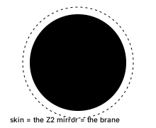
The stage: a 4-ball with a 3-sphere skin
A 4-dimensional ball whose 3-sphere skin is the Z2 mirror — the brane. Nothing lies beyond it: the dashed "outside" is our own bulk in reflection. Everything we call cosmology happens on and in that skin.
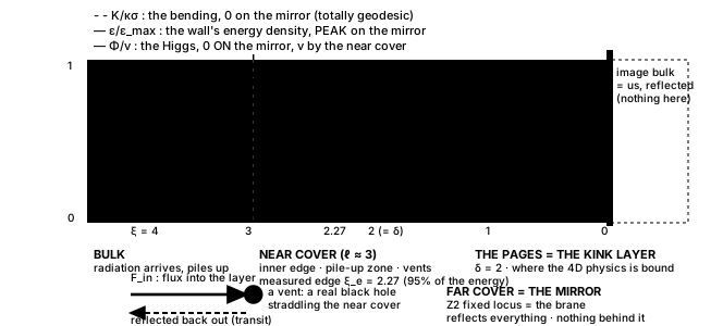
The layer, measured: three profiles across the wall
Reading right to left, the way the bulk sees it: the Higgs field Φ (green) climbs from zero on the mirror to its vacuum value by the near cover; the wall's energy density ε (amber) peaks exactly on the mirror; the bending K (blue, dashed) is zero on the mirror — totally geodesic — and rises to the thin-wall value only at the near cover. The measured edge of the layer sits at ξ_e = 2.27, against a tanh scale δ = 2.
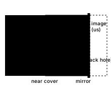
The wall is a layer, not a surface
Bulk → near cover (the pile-up zone, where vents form) → the pages (the Higgs kink, thickness δ = 2 in code units) → far cover = the mirror (the Z2 fixed locus; totally geodesic; reflects everything; nothing behind it). Resolved, not expanded — its gravitational thickness κσδ ≈ 1.4 rules out a thin-wall treatment.